
Distribution of the Component Scores
Notation
Step 9 gave us the component scores $\mathbf{z}_3 = \widetilde{\mathbf{Y}}_c\mathbf{W}_3$, one column per retained component (PC1, PC2, PC3), one row per observation.
In practice, to derive a stress, each column of $\mathbf{z}_3$ is treated as a sample from a distribution: the classical approach fits a normal distribution to each component's scores, using the sample mean $\mu_i$ and sample standard deviation $\sigma_i$ of that column. A stress at a given confidence level (e.g. 99.5th percentile for a 1-in-200 shock) is then read off that fitted distribution and mapped back through the loadings $\mathbf{W}_3$ to obtain a yield curve shock.
This is a fixed distribution — $\mu_i$ and $\sigma_i$ are point estimates from history, with no uncertainty attached to them. That is the aspect the Bayesian extension revisits later.
step 1 - plot the fitted distribution of each component's scores
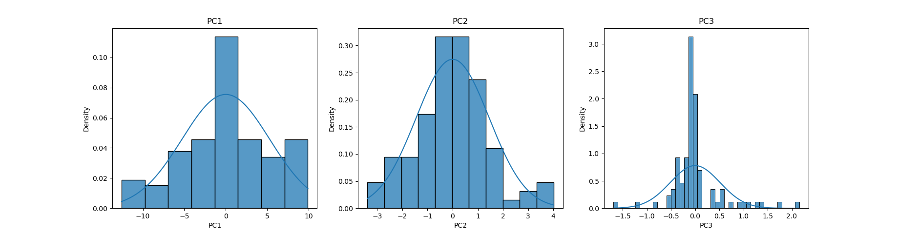
step 2 - chi-squared goodness of fit test
Tests whether each component's scores are consistent with the fitted normal ($\mu_i$, $\sigma_i$ estimated from that column). Scores are binned, observed counts compared against counts expected under the fitted normal's CDF, giving a $\chi^2$ statistic per component. Degrees of freedom are reduced by 2 (via ddof=2) since both $\mu_i$ and $\sigma_i$ were estimated from the same data rather than specified in advance. A low $p$-value indicates the normal fit is a poor description of that component's scores.
import subprocess
%run ./dataframes/step10_goodness_of_fit.py
%run ./dataframes/truncate_with_ellipsis.py
df = goodness_of_fit()
subprocess.run(['wl-copy'], input=truncate_with_ellipsis(df, 3).to_html(index=False).encode())
| component | chi2_statistic | p_value |
|---|---|---|
| PC1 | 17.274096 | 1.571173e-02 |
| PC2 | 16.009892 | 2.502614e-02 |
| PC3 | 87.040452 | 5.007683e-16 |
step 3 - sensitivity check with a different bin count
goodness_of_fit already takes n_bins as a parameter, so the check is a straight re-run with a different bin count rather than a code change — this checks whether the step 2 rejections (borderline for PC1/PC2) hold up under a different binning choice.
import subprocess
%run ./dataframes/step10_goodness_of_fit.py
%run ./dataframes/truncate_with_ellipsis.py
df = goodness_of_fit(n_bins=20)
subprocess.run(['wl-copy'], input=truncate_with_ellipsis(df, 3).to_html(index=False).encode())
| component | chi2_statistic | p_value |
|---|---|---|
| PC1 | 24.625169 | 1.034194e-01 |
| PC2 | 27.538499 | 5.062812e-02 |
| PC3 | 290.808524 | 8.844976e-52 |
Python
filename: step9_component_scores_distribution.py
from dataframes.step9_scores import *
import numpy as np
import seaborn
import matplotlib.pyplot as plt

'''
this code produces a chart showing the distribution of each component score,
with a fitted normal overlay (as used in practice to derive stresses)
see the create_snippets.py file for the one that calls this one.
'''

def component_scores_distribution_chart(filename):
    df = scores()
    pc_cols = [c for c in df.columns if c.startswith("PC")]
    fig, axes = plt.subplots(1, len(pc_cols), figsize=(18.4, 4.8))
    for ax, pc in zip(axes, pc_cols):
        seaborn.histplot(df[pc], stat="density", ax=ax)
        mu, sigma = df[pc].mean(), df[pc].std()
        x = np.linspace(df[pc].min(), df[pc].max(), 200)
        pdf = (1 / (sigma * np.sqrt(2 * np.pi))) * np.exp(-0.5 * ((x - mu) / sigma) ** 2)
        ax.plot(x, pdf)
        ax.set_title(pc)
    plt.savefig(filename)
    return
filename: step10_goodness_of_fit.py
from dataframes.step9_scores import *
from scipy import stats

def goodness_of_fit(n_bins=10):
    df = scores()
    pc_cols = [c for c in df.columns if c.startswith("PC")]
    results = []
    for pc in pc_cols:
        x = df[pc].values
        mu, sigma = x.mean(), x.std()
        counts, bin_edges = np.histogram(x, bins=n_bins)
        cdf_edges = bin_edges.copy()
        cdf_edges[0], cdf_edges[-1] = -np.inf, np.inf
        cdf_vals = stats.norm.cdf(cdf_edges, mu, sigma)
        expected = len(x) * np.diff(cdf_vals)
        chi2_statistic, p_value = stats.chisquare(counts, expected, ddof=2)
        results.append({
            "component": pc,
            "chi2_statistic": chi2_statistic,
            "p_value": p_value,
        })
    return pd.DataFrame(results)